In preparation for the SCALE and Open San Diego Crime ANalysis Presentation, I downloaded the data package for the presentation and started on the analysis a bit early.
The presentation will use the San Diego Police 2015 calls for service, but the data repository has 2016 and 2017 as well. The seperate files for each of the three years are converted into a data package on our repository, and I also created Metapack packages for the boundary files for beats, neighborhoods and districts. Merging in these boundary files allows for analysing crime counts by geography. Here are the packages:
This notebook requires the metapack package for downloading URLS, which you should be able to install, on Python 3.5 or later, with pip install metapack
%matplotlib inline
import metapack as mp
import pandas as pd
import seaborn as sns
import matplotlib.pyplot as plt
import geopandas as gpd
The Metapack system allows for packaging data, long with all of the metadata, and the open_package function can be used to load packages off the web. The the URL below is to a CSV package, which just referrs to CSV files on the web. You can get the link by to the CSV package file from the resource for sandiego.gov-police_regions-1 in the SRDRL data library repository page for the package
regions = mp.open_package('http://library.metatab.org/sandiego.gov-police_regions-1.csv')
regions
San Diego Police Regions
sandiego.gov-police_regions-1
Boundary shapes for San Diego neighborhoods, beats and divisions.
metapack+http://library.metatab.org/sandiego.gov-police_regions-1.csv
Contacts
Wrangler: Eric Busboom Civic Knowledge
Resources
- pd_beats – http://library.metatab.org/sandiego.gov-police_regions-1/data/pd_beats.csv Police beats
- pd_divisions – http://library.metatab.org/sandiego.gov-police_regions-1/data/pd_divisions.csv Police Divisions
- pd_neighborhoods – http://library.metatab.org/sandiego.gov-police_regions-1/data/pd_neighborhoods.csv Police Neighborhoods
After opening packages, we can ask the package for what resources it has, download those resources, and turn them into Pandas dataframes.
calls_p = mp.open_package('http://library.metatab.org/sandiego.gov-police_calls-2015e-1.csv')
calls_p
Police Calls for Service
sandiego.gov-police_calls-2015e-1
Calls dispatched by the San Diego Police Department’s communications dispatch
metapack+http://library.metatab.org/sandiego.gov-police_calls-2015e-1.csv
Contacts
Wrangler: Eric Busboom Civic Knowledge
Resources
- call_type – http://library.metatab.org/sandiego.gov-police_calls-2015e-1/data/call_type.csv Type of call
- disposition – http://library.metatab.org/sandiego.gov-police_calls-2015e-1/data/disposition.csv Classification
- beat – http://library.metatab.org/sandiego.gov-police_calls-2015e-1/data/beat.csv San Diego PD Beat
- pd_calls – http://library.metatab.org/sandiego.gov-police_calls-2015e-1/data/pd_calls.csv Combined pd_calls for 2015, 2016 and YTD 2017
References
- pd_calls_2015 – http://seshat.datasd.org/pd/pd_calls_for_service_2015_datasd.csv Service calls for 2015
- pd_calls_2016 – http://seshat.datasd.org/pd/pd_calls_for_service_2016_datasd.csv Service calls for 2016
- pd_calls_2017_ytd – http://seshat.datasd.org/pd/pd_calls_for_service_2017_datasd.csv Service calls for 2017, Year To Date
calls_r = calls_p.resource('pd_calls')
calls_r
pd_calls
| Header | Type | Description |
|---|---|---|
| incident_num | text | Unique Incident Identifier |
| date_time | datetime | Date / Time in 24 Hour Format |
| day | integer | Day of the week |
| stno | integer | Street Number of Incident, Abstracted to block level |
| stdir1 | text | Direction of street in address |
| street | text | Name of Street |
| streettype | text | Street Type |
| stdir2 | text | If intersecting street available, direction of that street |
| stname2 | text | If intersecting street available, street name |
| sttype2 | text | If intersecting street available, street type |
| call_type | text | Type of call |
| disposition | text | Classification |
| beat | integer | San Diego PD Beat |
| priority | text | Priority assigned by dispatcher |
call_type_r = calls_p.resource('call_type')
call_types = call_type_r.dataframe().rename(columns={'description':'call_type_desc'})
call_types.head()| call_type | call_type_desc | |
|---|---|---|
| 0 | 10 | OUT OF SERV, SUBJTOCALL |
| 1 | 10-97 | ARRIVE ON SCENE |
| 2 | 1016 | PRISONER IN CUSTODY |
| 3 | 1016PT | PTU (PRISONER TRANSPORT) |
| 4 | 1016QC | SHOPLIFTER/QUICK CITE |
regions_r = regions.resource('pd_beats')
regions_r
pd_beats
| Header | Type | Description |
|---|---|---|
| id | integer | |
| objectid | integer | |
| beat | integer | |
| div | integer | |
| serv | integer | |
| name | text | |
| geometry | geometry |
# The beats.cx[:-116.8,:] bit indexes the bounding box to exclude the empty portion of the
# county. San Diego owns the footprint of a dam in east county, which displays as a tiny
# dot in the middle of empty space.
# Note that this isn't actually defininf the bounding box; it's cutting out far-east regions,
# and then GeoPandas creates the smaller bounding box that excludes them. So, the actually
# value in the cx indexder can vary a bit.

# Converting to float makes merging with the calls df ewasier, since the beat column
# in that df has nans.

beats = regions_r.dataframe().geo
beats['beat'] = beats.beat.astype(float)
beats = beats.set_index('beat').cx[:-116.55,:]
beats.plot();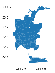
There are a lot of interesting patterns in crime data when you create heat maps of two time dimensions, a visualization called a “Rhythm Map”. We’ll add the time dimensions now for use later.
pd_calls = calls_r.read_csv(low_memory=False)

def augment_time(df):
    df['date_time'] = pd.to_datetime(df.date_time)

    df['hour'] = df.date_time.dt.hour
    df['month'] = df.date_time.dt.month
    df['year'] = df.date_time.dt.year
    df['dayofweek'] = df.date_time.dt.dayofweek
    df['weekofyear'] = df.date_time.dt.weekofyear

    df['weekofdata'] = (df.year-df.year.min())*52+df.date_time.dt.weekofyear
    df['monthofdata'] = (df.year-df.year.min())*12+df.date_time.dt.month

    return df

assert pd_calls.call_type.dtype == call_types.call_type.dtype

pd_calls = augment_time(pd_calls).merge(call_types, on='call_type')

pd_calls['beat'] = pd_calls.beat.astype(float)

pd_calls = pd_calls.merge(beats.reset_index()[['beat', 'name']], on='beat')\
    .rename(columns={'name':'beat_name'})
Incident Count Maps
The following maps plot the counts of incidents, over the whole dataset, for different call types, per beat. As is familiar to anyone who has worked with San Diego area crime data, the host spots for most incident types are Pacific Beach and Downtown.
def plot_geo(df, color_col, title=None):
    # Need to get aspect right or it looks wacky
    bb = beats.total_bounds
    aspect = (bb[3] - bb[1])/ (bb[2]-bb[0])
    x_dim = 8

    fig = plt.figure(figsize = (x_dim,x_dim*aspect))
    ax = fig.add_subplot(111)

    df.plot(ax=ax,column=color_col, cmap='RdYlGn_r',
                     scheme='fisher_jenks', legend=True);

    if title:
        fig.suptitle(title, fontsize=18);

    leg = ax.get_legend()

    #leg.set_bbox_to_anchor((0., 1.02, 1., .102))
    leg.set_bbox_to_anchor((1,.5))

    plt.tight_layout(rect=[0, 0.03, 1, 0.95])

_ = gpd.GeoDataFrame(pd_calls.groupby('beat').incident_num.count().to_frame()\
                               .join(beats))

plot_geo(_, 'incident_num', 'Incidents Per Beat, 2015 to Aug 2017')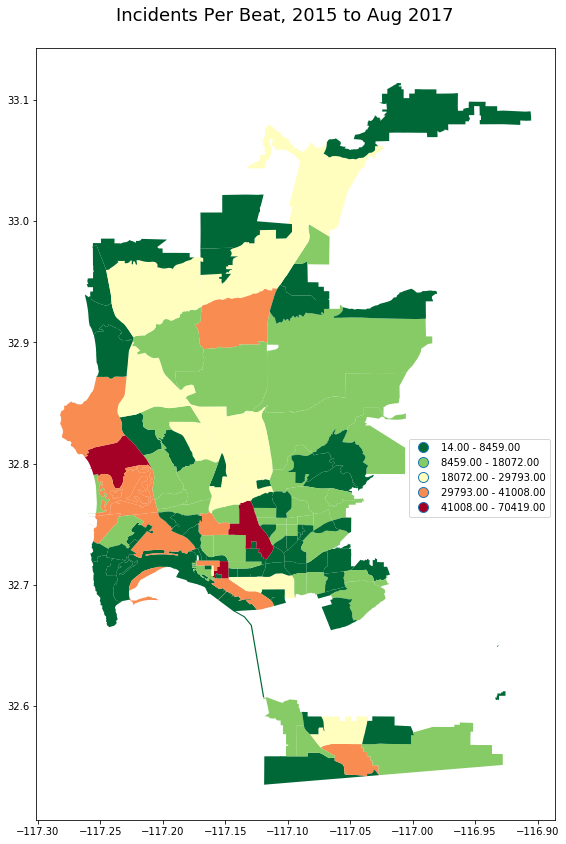
pd_calls.call_type_desc.value_counts().iloc[10:30]FLAG DOWN/FIELD INITIATED 28280
REQUEST FOR TOW TRUCK 27274
NO DETAIL ACCIDENT 27070
MENTAL CASE 25779
SPECIAL DETAIL 25115
SELECTIVE ENFORCEMENT 25098
FOLLOW-UP BY FIELD UNIT 24348
HAZARDOUS CONDITION 23954
SLEEPER 21584
INFORMATION FOR DISPATCHERS 21490
TRAFFIC STOP,FOR TMPOUT 19084
ALL UNITS INFORMATION-PRI 2 19056
LOUD PARTY 17803
CAR THEFT REPORT 16952
VEH VIOLATING 72HR PARKING RES 16155
BATTERY 15757
RECKLESS DRIVING-ALL UNITS 15197
CRIME CASE NUMBER REQUEST 15122
FOOT PATROL/FIELD INITIATED 14955
BURGLARY REPORT 14652
Name: call_type_desc, dtype: int64
_ = gpd.GeoDataFrame(pd_calls[pd_calls.call_type_desc == 'LOUD PARTY']
                             .groupby('beat')
                             .incident_num.count().to_frame()\
                             .join(beats))

plot_geo(_, 'incident_num', "LOUD PARTY calls, 2015 to Aug 2017") 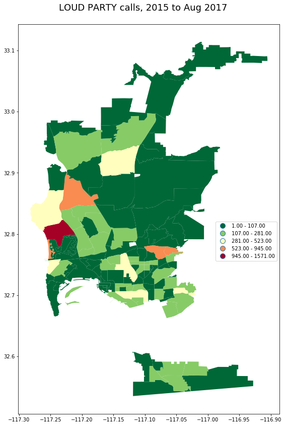
_ = gpd.GeoDataFrame(pd_calls[pd_calls.call_type_desc == 'ILLEGAL PARKING']
                             .groupby('beat')
                             .incident_num.count().to_frame()\
                             .join(beats))

plot_geo(_, 'incident_num', "ILLEGAL PARKING calls, 2015 to Aug 2017") 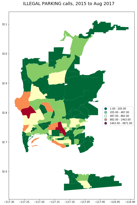
_ = pd_calls[pd_calls.call_type_desc == 'BATTERY']\
                             .groupby('beat')\
                             .incident_num.count().to_frame()\
                             .join(beats)


plot_geo(gpd.GeoDataFrame(_), 'incident_num', "BATTERY calls, 2015 to Aug 2017") 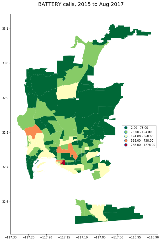
Sometimes, very high density areas like PB and Downtown will obscure patterns in other areas. One of the ways to handle this is to just exclude those areas. First, let’s locate which are the highest crime area.
_.sort_values('incident_num', ascending=False).head(10)| incident_num | id | objectid | div | serv | name | geometry | |
|---|---|---|---|---|---|---|---|
| beat | |||||||
| 521.0 | 1278 | 98 | 489 | 5 | 520 | EAST VILLAGE | POLYGON ((-117.1508808796175 32.71942332829821… |
| 122.0 | 738 | 64 | 231 | 1 | 120 | PACIFIC BEACH | POLYGON ((-117.2221709033007 32.81525925531844… |
| 524.0 | 695 | 93 | 463 | 5 | 520 | CORE-COLUMBIA | POLYGON ((-117.171021304813 32.71987375185346,… |
| 523.0 | 654 | 30 | 83 | 5 | 520 | GASLAMP | POLYGON ((-117.1610808948147 32.71569562856276… |
| 627.0 | 565 | 83 | 408 | 6 | 620 | HILLCREST | POLYGON ((-117.1616090022237 32.75878799862505… |
| 813.0 | 495 | 74 | 352 | 8 | 810 | NORTH PARK | POLYGON ((-117.1304627884029 32.7691214134209,… |
| 512.0 | 368 | 58 | 203 | 5 | 510 | LOGAN HEIGHTS | POLYGON ((-117.1213484238577 32.70672846114386… |
| 614.0 | 350 | 24 | 64 | 6 | 610 | OCEAN BEACH | POLYGON ((-117.2340495278368 32.75789474471601… |
| 511.0 | 348 | 21 | 52 | 5 | 510 | None | (POLYGON ((-117.2252864171211 32.7026041543147… |
| 511.0 | 348 | 132 | 626 | 5 | 510 | BARRIO LOGAN | POLYGON ((-117.1527936937041 32.70523801385234… |
Here is the map excluding the top 5 high crime areas. The excluded areas are omitted completely, shown in white.
# Could also get the beats by name.
pb_beat = beats[beats.name=='PACIFIC BEACH'].index.values[0]
gas_beat = beats[beats.name=='GASLAMP'].index.values[0]

low_crime = _.sort_values('incident_num', ascending=False).iloc[5:]
_lc = _.loc[list(low_crime.index.values)]

plot_geo(gpd.GeoDataFrame(_lc), 'incident_num',
"BATTERY calls, 2015 to Aug 2017, Lower Crime Areas") 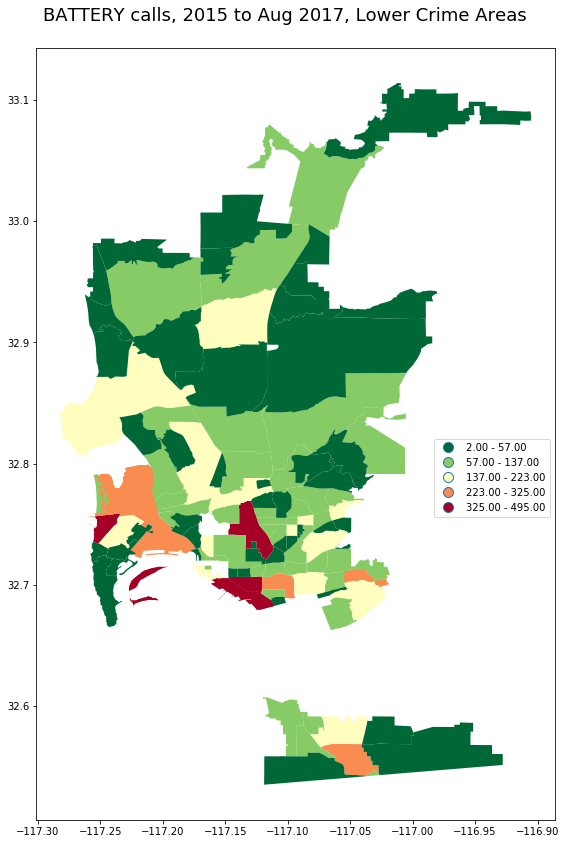
_ = gpd.GeoDataFrame(pd_calls[pd_calls.call_type_desc == 'BATTERY']
                             .groupby('beat')
                             .incident_num.count().to_frame()\
                             .join(beats))

plot_geo(_, 'incident_num', "BATTERY calls, 2015 to Nov 2017") 
_ = gpd.GeoDataFrame(pd_calls[pd_calls.call_type_desc == 'MENTAL CASE']
                             .groupby('beat')
                             .incident_num.count().to_frame()\
                             .join(beats))

plot_geo(_, 'incident_num', "MENTAL CASE calls, 2015 to Aug 2017") 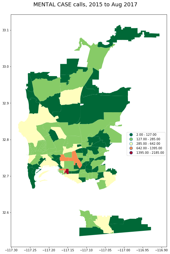
Rhythm Maps
By plotting two time dimensions in a heat map we can often see interesting patterns.
Here we’ll look at the rhythm of parties in Pacific Beach, plotting the number of party calls as colors in a maps with an X axis of the day of the week, and a Y axis of the hour of the day. As you’d expect, the LOUD PARTY calls are primarily on Friday and Saturday nights.
pb_beat = beats[beats.name=='PACIFIC BEACH'].index.values[0]

_ = pd_calls[(pd_calls.call_type_desc=='LOUD PARTY') & (pd_calls.beat == pb_beat)]

ht = pd.pivot_table(data=_,
                    values='incident_num', index=['hour'],columns=['dayofweek'],
                    aggfunc='count')

fig, ax = plt.subplots(figsize=(6,6))

sns.heatmap(ht, ax=ax);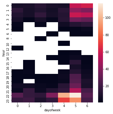
Looking at the hour of day versus month, there is a clear seasonal pattern, with fewer loud party calls during the winter.
pb_beat = beats[beats.name=='PACIFIC BEACH'].index.values[0]

_ = pd_calls[(pd_calls.call_type_desc=='LOUD PARTY') & (pd_calls.beat == pb_beat)]


fig, ax = plt.subplots(figsize=(8,8))

fig.suptitle("LOUD PARTY Calls In Pacific Beach\n2015 to Aug 2017\nBy Hour and Month", fontsize=18);

sns.heatmap(ht, ax=ax);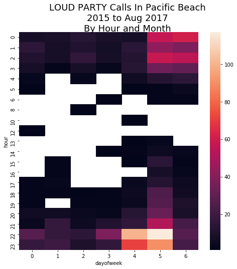
hm_beats = pd_calls[['beat_name', 'hour','month']].copy()
hm_beats['count'] = 1
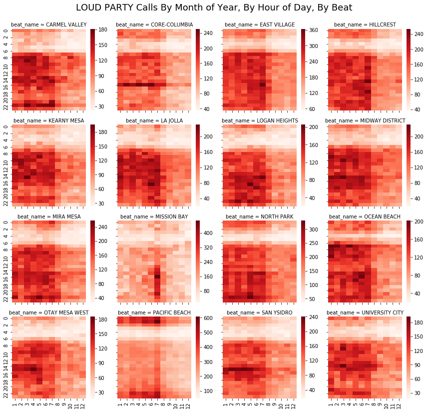
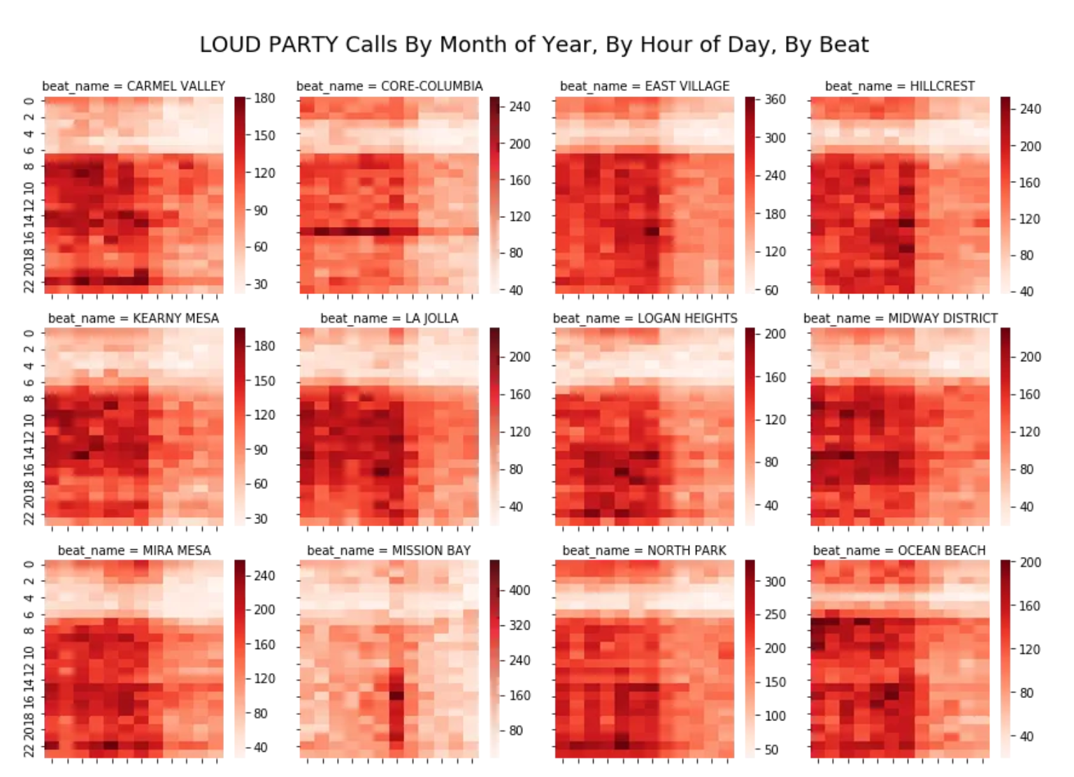
hm_beats = hm_beats.groupby(['beat_name', 'hour','month']).count().reset_index()Small Multiple Rhythm Maps
Rhythm maps really shine when they are part of a small multiple grid, or in Seaborn terminology, a Facet Grid. These take a bit more work to setup, but they are really valuable for finding patterns.
Note how clearly you can see when students go back to school, and the July rowdiness in PB and MB.
But, the really interesting thing is that in many communities, most obviously in San Ysidro, Core-Columbia, Otay Mesa, and a few others, there are a high number of calls are 4:00 in the afternoon. Any ideas?
# Top 16 beats
top_beats= pd_calls.beat_name.value_counts().index.values[:16]

from IPython.display import display

# select only the rows for the top 16 beats
_ = hm_beats[hm_beats.beat_name.isin(top_beats)]

g = sns.FacetGrid(_, col="beat_name", col_wrap=4)

def facet_heatmap(data,  color, **kwargs):

    ht = data.pivot(index="hour", columns='month', values='count')

    sns.heatmap(ht, cmap='Reds', **kwargs)

#cbar_ax = g.fig.add_axes([.92, .3, .02, .4])  # Create a colorbar axes


with sns.plotting_context(font_scale=3.5):
    g = g.map_dataframe(facet_heatmap)

plt.tight_layout(rect=[0, 0.03, 1, 0.95])
g.fig.suptitle("LOUD PARTY Calls By Month of Year, By Hour of Day, By Beat",
              fontsize=18);