

Eric Busboom.
An isochrone ( meaning “equal time” ) is an area that encloses the points one can travel to in a fixed time. For a bird, an isochrone would be a circle, but humans usually have to follow roads, so human isochrones have shapes that mirror the road network. Despite the name, isochrones are most often computed using a fixed distance. For instance, a 5km isochrone would be all the points that are within 5km of a point, but using distances based on a road network, not the straight distance. So, instead of a 5km radius circle, a 5km isochrone will have a non-circular shape.
Civic Knowledge is developing a Python program for raster-based spatial analysis. The system can create isochrone regions, rasterize them, and use them in algebraic equations with other rasters, allowing for very powerful spatial analysis.
For a quick example, here is a 10km isochrone around Franklin Barbeque in Austin Texas.
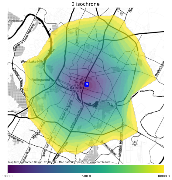
The isochrone region is colored by the distance from the central point, in meters. The area is computed by tracing the road network, then finding a region ( a concave hull ) that encloses all of the nodes ( the ends of road segments ) that are a specific distance from the central point. The distances are quantized to 500 meters.
There are a lot of analyses that we can do with this shape. One that is particularly interesting to a business is to calculate the number of customers in the area around the store, weighted by how likely they are to visit, which is a function of the attractiveness of the location and the distance from each consumer. The most common model for this sort of analysis is the Huff model:
$$P_{ij}= \frac{A_j^\alpha D_{ij}^{- \beta}} {\sum_{j=1}^{n}A_j^{\alpha} D_{ij}^{- \beta}}$$
where :
- $A_j$ is a measure of attractiveness of store
j - $r_{ij}$ is the distance from the consumer’s location,
i, to storej. - $\alpha$ is an attractiveness parameter
- $\beta$ is a distance decay parameter
- $n$ is the total number of stores, including store
j
The term $A_j^\alpha D_{ij}^{- \beta}$ multiplies the “attractiveness” of the location times the distance weighted probability of the consumer visiting the location. The attractiveness term, $A_j^\alpha$ can be any of a variety of measures, but retail square footage is a common one. The exponent $\alpha$ accounts for the non-linearity of attractiveness; a store that has twice the square footage is not always twice as attractive.
The distance weighting value, because of it’s negative exponent, accounts for consumers who are farther away being less likely to visit. If $\beta$ is 1, then the term reduces to $1/r$ for distance $r$ and if $\beta$ is two, the term is $1/r^2$. Because $1/r^2$ is the same law that gravity follows, this model is sometimes called Huff’s Gravity Model.
While the Huff model is expressed as the probability that a consumer will visit a location, we can also use it to determine the likely number of visitors to a location, by calculating the value for every person in the retail cachement area. For this analysis, we will use a raster map of population density. Here is the map of population, based on census tracts for 2019, for the area around our location.
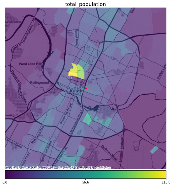
Each pixel of the map is 100m square and the value at the pixel is the estimated number of people who live in that square, computed by dividing the total estimated population of a census tract by its area. By calculating the Huff model value for each pixel and multiplying by the number of people in that pixel, then summing over all pixels, we can get an estimated number of visitors to the location.
This calculation will involve these steps:
- Compute the isochrone for the location, with pixel values of meters distance from the central location.
- Set ${\beta}=1$ and compute $1/r$ for all pixels.
- Multiply $1/r$ values by the population.
- Sum the values to get an estimate of the number of customers.
For this example, we are only working with one location, and assuming the atractiveness is 1. For the full Huff model we would have to perform this calculation for every location, sum the results and use it as a denominator.
The original isochrone values are in meters from the central point and we use ${\beta}=1$ so the weighting for population will be $1/r$. Then we can multiply the weighting by the population to get a weighted population.

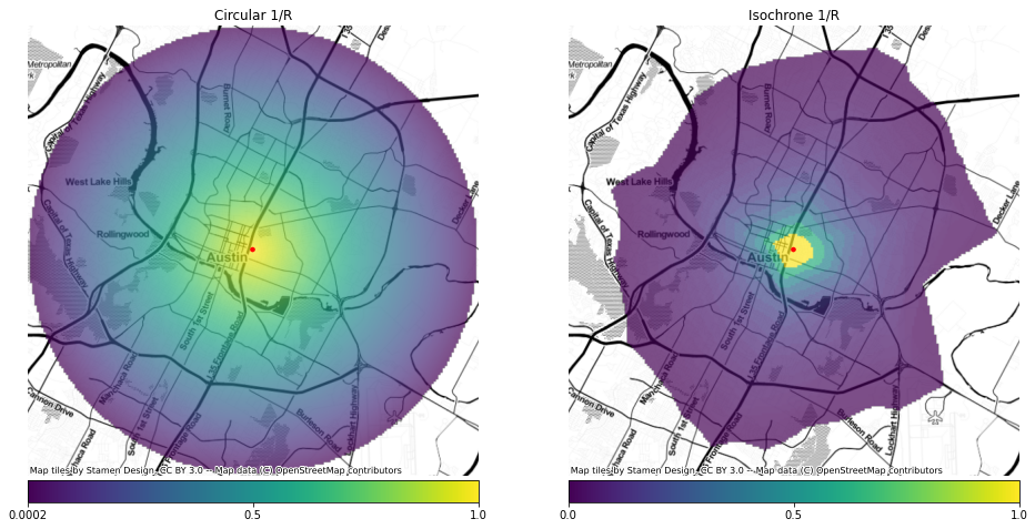
The total population of the whole isochrone area is 383,044 but the weighted population within the isochrone is 43,005. The difference is the result of the $1/r$ weighting, which counts population farther away with a value less than population that is closer. If we had used the straight line distance instead of the isochrone — which would be a circle instead of the odd isochrone shape — the 1/r weighted population would be 192,230.
Here is what the straight-line distances look like versus the isochrone; they are very different.
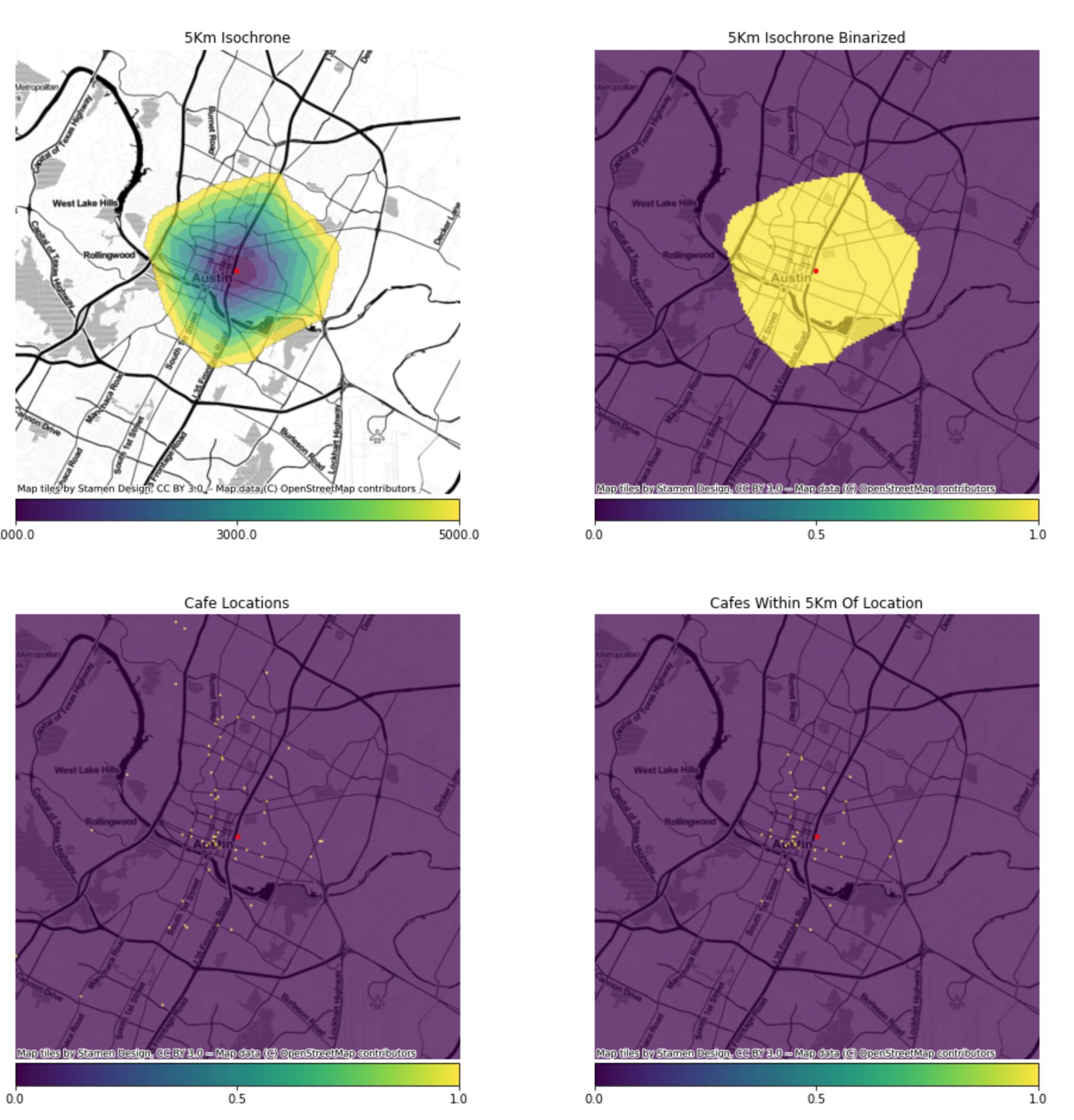
We can also use the isochrones to count the number of specific sites, such as related businesses or competitors, withiWe can also use the isochrones to count the number of specific sites, such as related businesses or competitors, within a given area. In this case, we will create a raster of the locations of cafes, which will have a value of 1 where there is a cafe and 0 elsewhere. We’ll binarize the isochone areas where the value is less than 5_000, which will produce a raster with 1 for the cells that are 5km or less away from the central point, 0 elsewhere. Multiplying these two rasters will produce a raster with a value of 1 where there is a cafe that is 5km or less from the central point, and summing the values of that raster produces a count of cafes.
Isochrone areas are a powerful addition to your spatial analysis techniques, allowing a more accurate assessment of cachement areas. Using isochrones can produce significantly different results that simplier fixed radii, although they can require more effort to use, particualrly in a vector-based process. However, when used as part of a raster-based spatial analysis, there is little difference.