Eric Busboom.
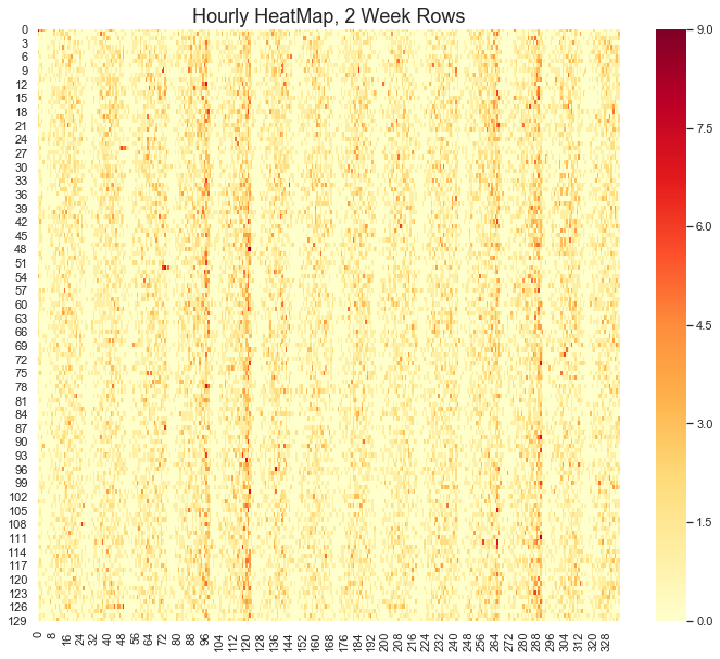
A Rhythm map is a heat map with two time dimensions, which makes it much esier to find temporal patterns in some kinds of data. This example will use crime incidents from San Diego county, from 2007 to 2013..
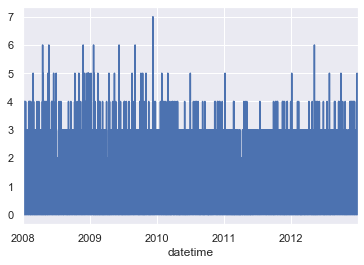
Plotting the number of incidents for burglary versus the hour of the day, for instance, results in this dull chart:
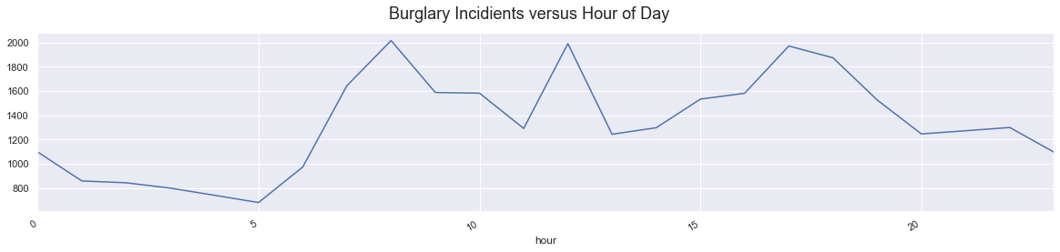
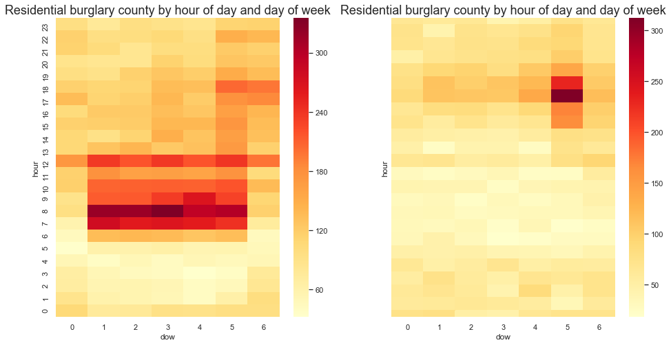
There are a few interesting patterns here, primarily the minimum at about 5:00AM. But nearly all categories of crime have a lull at 5:00 in the morning, which isn’t very surprising. Part of the reason that the chart isn’t very useful is that there are several types of burglarly, and they happen at different times of the week and different times of the day, a distinction which isn’t visible in a line plot. So, let’s look at burglary by hour of day and day of week.
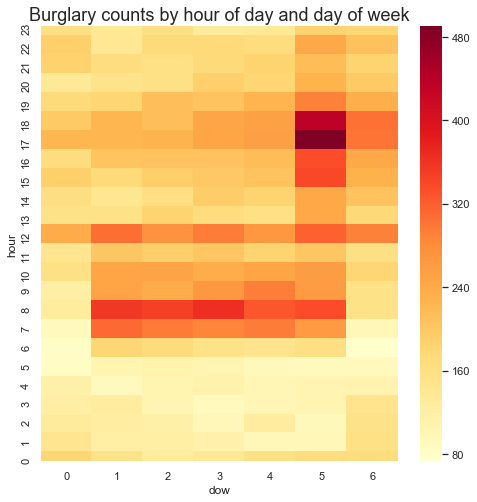
Here we can see three patterns:
- A strong line at noon. This is an artifact of data collection; reports without a time probably default to noon.
- A cluster in the mornings and afternoons of weekdays. These are residential burglaries.
- A strong line in the early evening on Fridays; These are commercial burglaries.
Here are the residential and commercial burglaries broken out.
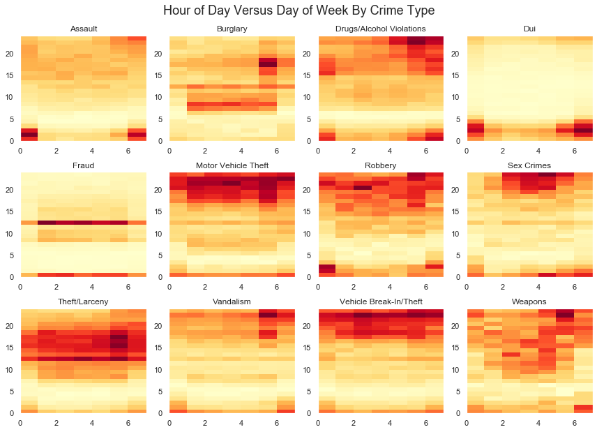
There are many different patterns like these for the different crime categories.

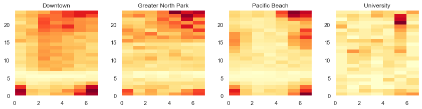
There are also different patterns for a single crime type for different communities. Alcohol violations in Downtown are very late on weekends, and much earlier on weekdays, while in Pacific Beach, the violations are more concentrated earlier on weekends, and UCSD students only get rowdy on Friday.
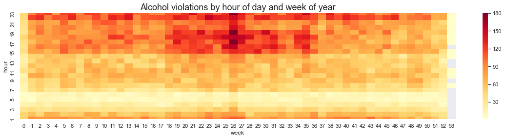
Here is another interesting pattern in alcohol violations, when plotted by hour of day versus week of year: they are more common in the summers and more common after 3:00PM, except for week 27 — the typical week of July 4 — when the violations are spread through the entire day.
There are many other patterns to be found in crime dataset by looking at other combinations of time units, community, and crime type. If you’d like to explore some of these patterns, you can clone, run and extend this notebook from github.
<matplotlib.axes._subplots.AxesSubplot at 0x7fe5923feba8>
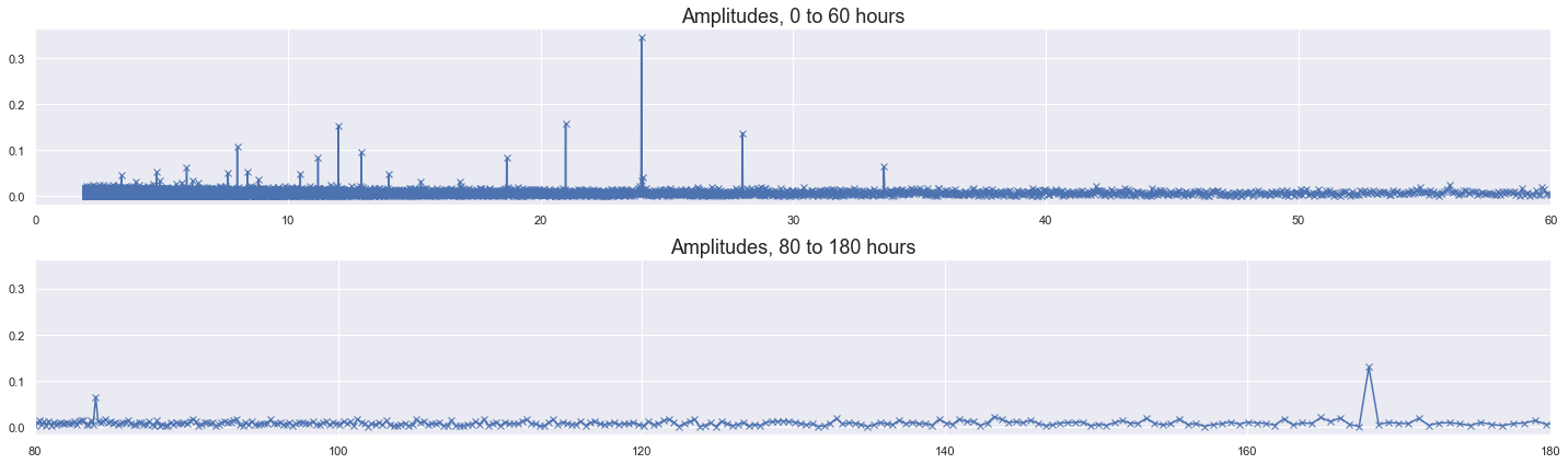
| freq | amp | |
|---|---|---|
| period | ||
| 23.998905 | 0.041669 | 0.346067 |
| 20.999042 | 0.047621 | 0.158237 |
| 11.999453 | 0.083337 | 0.153824 |
| 27.998723 | 0.035716 | 0.137281 |
| 167.992337 | 0.005953 | 0.129606 |
| 7.999635 | 0.125006 | 0.106893 |
| 12.922487 | 0.077384 | 0.095370 |
| 18.665815 | 0.053574 | 0.083372 |
| 11.199489 | 0.089290 | 0.082961 |
| 83.996169 | 0.011905 | 0.064842 |
| 33.598467 | 0.029763 | 0.064258 |
| 5.999726 | 0.166674 | 0.062298 |
| 8.399617 | 0.119053 | 0.053870 |
| 4.799781 | 0.208343 | 0.052602 |
| 7.636015 | 0.130958 | 0.050812 |